iSTREAM Performance Investigator (PI) is a specialised tool for collecting and analysing job performance data, designed to tackle intricate performance issues through a single data collection approach. PI acts as a versatile umbrella tool, efficiently coordinating with other collectors while providing a unified interface for the comprehensive analysis of all gathered data. This unique capability ensures a streamlined and efficient process, allowing users to address complex performance challenges seamlessly after a single collection process run.

PI’s unique features include:

• Open Data Collection Model: encompassing job and thread polling data retrieved through IBM i Work Management APIs, Collection Services (STRPFRT) data, Job Watcher data, Disk Watcher data, SQL Performance Monitor (DBMON) data, and selected PEX summary data.
• Single Data Collection Engine: targeting a group of jobs for a cohesive and efficient data gathering process.

• Performance Monitor: Identifying “runaway” jobs based on predefined rules and utilising the above collectors for data gathering.

• Unified Data Analysis Interface: comprising two components – a 5250 analysis interface (text only) and an MS Windows analysis interface leveraging open Microsoft Excel forms for additional totaling and graph building.

Using iSTREAM PI, all analytical queries are executed through open Query Manager queries and, optionally, Microsoft Excel sheets and graphs.

Full utilisation of PI functionality requires the installation and licensing of the iSTREAM Access for MS Windows option.

One of the most efficient methods for improving long-running batch performance on the IBM i platform is multistreaming, involving the submission of multiple instances of the processing program, each handling its own subset of data. Typically, this is achieved by creating a multistreaming wrapper around the original process. While there are various approaches to implement multistreaming, regardless of the chosen method, it requires addressing three key questions and selecting from the associated sets of options.

Question 1. What is the runtime model employed?

Two options are available in this context: submitting processing streams as batch jobs or threads. The latter method is seldom used and, in reality, provides few advantages. While it is true that threads typically consume fewer resources, the difference in the case of, for instance, 10 threads versus 10 jobs for a 30-minute batch is negligible. Additionally, the thread model implies thread-safety of the processes, a criterion met by very few legacy batch programs.

Question 2. What mechanisms are utilised to logically partition the processed data?

This option presents a more interesting choice. The widely adopted approach involves the creation of temporary data subsets, one for each stream. While this method is applicable excluisively to read-only data and requires additional time and resources for subset creation, it continues to be the preferred option for many IBM i users.

A dynamic modification of this approach involves the creation of a conveyor mechanism, similar to the mapping procedure in the MapReduce programming model. The conveyor retrieves data from primary files (tables) and subsequently conducts filtering and sorting into queues associated with the active stream processes. To implement this method, the original batch programs typically need modification to receive data from queues instead of directly from files (tables).

The second method relies on the OPNQRYF command. In this approach, each stream executes the command with a unique filter and subsequently overrides the program’s primary file file with the the query file. This method is effective for both physical and logical primary files, but it is suited for OPM and ILE native data access only.

If the access to the primary datasets of the process relies on the use of SQL, a more suitable approach involves constructing temporary views with appropriate selections, one for each stream, and subsequently overriding the primary tables/views in the batch process with these views. However, similar to the previous method, this approach has its drawbacks—it is not compatible with OPM and ILE native access programs utilising keyed logical files, making it less universal in its applicability.

The most comprehensive approach is to generate temporary views, one for each stream, and then execute OPNQRYF commands for retrieving or updating the data in those views. This method stands out as the optimal way to manage heterogeneous batch processes that employ both native and SQL data access.

Question 3. What types of data breakdown are most suitable for the given process?

Relative record number (RRN)

The most straightforward file or table breakdown involves splitting data by the relative record number. Each stream is assigned an equal range of record numbers for processing, making it effective even with logical files and views. However, the challenge lies in achieving a truly balanced breakdown. In cases with a substantial number of deleted records in a file, some streams may be allocated significantly larger volumes than others.

Another drawback of the RRN breakdown is its potential incompatibility with the algorithm employed by the batch process. For instance, if the process is configured to calculate totals by branch or region, all records corresponding to a particular branch or region must be allocated to the same stream. This is a requirement that the RRN breakdown clearly violates.

Field (column) value ranges

A good method in this scenario involves breaking down the data by values of a specific database file (table) field (column). For instance, cost centers with IDs from 0001 to 1000 may be allocated to the first stream, 1001 to 2000 to the second, and so forth. While this approach enhances compatibility with the batch process algorithm compared to the RRN breakdown, it does come with its own set of drawbacks.

Firstly, defining groups of key value ranges for multistreaming may present a challenge. In many cases, this activity is manual and, moreover, needs to be periodically repeated to account for the dynamic nature of the values of the key field (column).

Secondly, achieving volume balancing in this scenario can be even more challenging. It is possible that the ‘head office cost centre’ of the company accumulates more business volumes than all other cost centers combined. In such cases, breaking down by cost centre ranges may not significantly contribute to effective multistreaming, as a majority of the batch processing could end up being allocated to a single processing stream.

Virtual field (column) value ranges

An interesting alternative for defining the breakdown is by the values of a virtual field or column. The concept of a virtual field-based breakdown is straightforward in theory, although the actual implementation may introduce complexities.

Elaborating on this approach, consider a scenario where a chosen physical or logical file selected for splitting includes an additional decimal field. The values of this field for various records are randomly assigned within the 1-999 range but remain consistently identical for records sharing a specific key, such as, for example, the cost centre number. In this setup, streams can be allocated based on the values of this virtual field. The random nature of the values in the virtual field might assist in auto-balancing to a signigficant extent.

One of the possible ways to implement the virtual field multistraming is as follows.

1. Create a new table, VFMS, with two columns: the key from the primary table, chosen for grouping the records into streams, and a decimal (3,0) field designated for the virtual field implementation.

CREATE TABLE VFMS(KEY1 CHARACTER (10 ) NOT NULL WITH DEFAULT,
VFIELD DECIMAL (3 , 0) NOT NULL WITH DEFAULT)

where KEY1 is the key selected.

2. Before initiating each batch run, ensure the worktable content is up-to-date, i.e. in sync with the data in the primary table, by executing the following SQL statements.

DELETE FROM VFMS B WHERE NOT EXISTS(SELECT * FROM PRIMARY A WHERE a.KEY1=b.KEY1)

INSERT INTO VFMS SELECT DISTINCT KEY,0 FROM PRIMARY A WHERE NOT EXISTS(SELECT * FROM VFMSWORK B WHERE a.KEY1=b.KEY1)

UPDATE VFMS SET VFIELD=INT(ABS(RAND()-0.000001)*999+1) WHERE VFIELD=0

The VFMS table can now be seamlessly joined with the PRIMARY table using the values of the KEY1 field, establishing the foundation for the virtual field implementation.

At runtime, the subsequent statement would be executed for each stream:

CREATE VIEW QTEMP/PRIMARY AS SELECT * FROM PRIMARY a WHERE ((EXISTS(SELECT * FROM VFMS B WHERE ( A.KEY1=b.KEY1)
AND (B.VFIELD >= lowerstreamlimit ) AND (B.VFIELD <= higherstreamlimit ))) OR ( NOT EXISTS(SELECT * FROM PRIMARY B WHERE ( A.KEY1=b.KEY1)))

This temporary view will then serve as the source for the data to be processed by the given stream.

3.  ROWNUMBER() function

A similar result can be achieved using the SQL OLAP ROW_NUMBER() function. This approach provides a notable benefit by obviating the necessity for an extra VFMS table. The randomisation of values for allocating records to a stream is executed by the SQL engine during the creation of the temporary view in QTEMP. However, the resulting SQL statements become somewhat intricate, rendering the generated code more challenging to comprehend and maintain.

4. Hiererchical data breakdown

At the pinnacle of sophistication lies the hierarchical breakdown approach, where the data in the primary table(s) is initially segmented by value ranges of a certain field (column), e.g. cost centre, and each range containing a single value undergoes further breakdown using either another field (e.g., account number), or a virtual field. This method exhibits a high probability of delivering a robust breakdown while still preserving compatibility with the batch algorithm.

Multistreaming, of course, presents other challenges, such as establishing the correct environment, including file overrides, QTEMP objects, and open files for each of the submitted process streams. Additionally, when the batch generates spool reports, careful consideration must be given to the optimal method of merging the spool files produced by the individual stream jobs.

All the previously mentioned methods and more are integral features of the iSTREAM LP Generic Multistreaming Option. This instrumental application is generally capable of multistreaming many existing batch processes without requiring any modifications to the original programs.

There are multiple file copy functions supported by the IBM i platform. They vary in the optional features offered, but regardless of the method used, file copying typically consumes time. The size of the files directly impacts the length of time a user must wait for the copy operation to be completed.

While the save-while-active feature may create the illusion of instant data copying for the initiator, the recipient of the copy still needs to wait for the background process to complete. SAN-based FlashCopy solutions can be seen as a step in the right direction, but they tend to be expensive, can be challenging to configure, and typically operate at the partition level rather than on individual files.

This gap in the fast file copy functionality is not inconsequential, and there is at least one specific use case that simply cries out for it.

Consider a traditional multi-regional ERP or banking system. Nowadays, these systems operate in a 24/7 mode while maintaining daily batch processing tasks, such as interest calculations, balance roll-ups, and inter-division settlements. To illustrate this operational model, we can use the following diagram.

Throughout the day, the primary system remains open for inquiries and data input. At a predefined time, the user input subsystem is temporarily suspended, and a copy of the key files is created. While the main system proceeds with its daily batch processing, the newly generated night library is utilized to serve divisions of the company operating in different time zones or customers.

The primary issue here is the downtime necessary to create a copy of files in the production library. For instance, a bank customer attempting to withdraw cash from an ATM during this time might receive a message like, “Your banking system is currently unavailable; please try again later.” The business usually requires a library copy to be completed within a very limited window, ideally within 2 minutes or less.While rebuilding the application to support queries and user input simultaneously during daily batch processing could be a possible solution, application owners often face significant constraints in this regard.

One solution worth considering is the iSTREAM File Replication feature. It follows a methodology similar to that of traditional HA/DR applications for IBM i, such as MIMIX or Maxava, hence its name. The method used involves creating a copy of the production files in advance, initiating file replication or synchronization, and by the time of the system swap, the files are effectively duplicated. The only remaining task is transitioning the user interfaces from the Day library to the Night library.

While the approach may not appear particularly original, there are several noteworthy distinctions between iSTREAM data replication and the replication methods implemented in the enterprise-level platforms mentioned earlier.

First, iSTREAM File Replication does not rely on journaling or journals.

Second, as a direct result of this, the need to duplicate the production library to match a particular journal entry for future replication is completely eliminated. Replication can start from the target files containing no records at all. This sets it apart from conventional journal-based High Availability/Disaster Recovery (HA/DR) systems, which often entail intricate and manual setup procedures.

Third, unlike journal-based object replication systems primarily designed for relatively static environments, where file and library deletion and recreation are exceptions, iSTREAM excels in managing these tasks treating them as routine operations.

Several other noteworthy features of iSTREAM File Replication include:

1. Transparent restart after replication errors, such as those related to locking.
2. Availability of APIs (implemented as CL commands) for all primary operations.
3. The ability to define the target file update strategy.
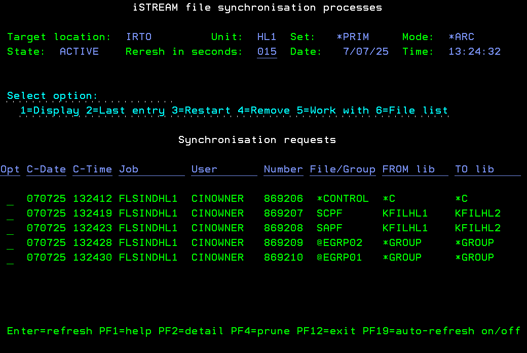
4. Interactive monitoring of replication, supported by APIs.

All in all, this feature of iSTREAM is an interesting cost-effective addition to the IBM i fast copy solutions family.

The most accurate description of the Save-While-Active (SWA) function that I could locate on the web is as follows: “The Save-While-Active function enables you to utilize your system while concurrently saving your IBM i system objects, in addition to integrating them seamlessly into your broader backup and recovery protocols.”

For some reason, comparisons between SWA and the SAN FlashCopy function are scarce, despite the fact that both essentially serve the same purpose and, more importantly, share very similar implementation methods.

While the save-while-active feature for backups has been available for many years, a significant number of customers remain hesitant to incorporate this parameter into their save commands. This hesitance was evident in 2010 when Tom Huntington made this observation in his article for MCPress Online, and regrettably, it continues to persist today.

There are at least two reasons for this hesitance. Firstly, there is a lack of understanding regarding the “point-in-time” copy concept. Many IBM i administrators believe that, although SWA backups can run concurrently with database updates by applications, the resulting backup doesn’t accurately represent the data at the specific point in time when the backup operation started. The second reason is the deceptive simplicity of the SWA feature.

Let’s consider an example of a traditional, long-running batch process.

/* BEFORE backup */
SAVOBJ OBJ(OBJ1 OBJ2… OBJn) LIB(APPLIB) DEV(xxxxxx)
/* Run batch proces */
CALL PGM(BATCH)
/* AFTER backup */
SAVOBJ OBJ(OBJ1 OBJ2… OBJn) LIB(APPLIB) DEV(xxxxxx)

If our primary concern is the duration of batch runtime, and a substantial portion of this duration is attributable to the time consumed by backups, then, setting aside any unwarranted doubts about the backup content, we might be tempted to merely add the SWA parameter to our backup requests:

/* BEFORE backup */
SAVOBJ OBJ(OBJ1 OBJ2… OBJn) LIB(APPLIB) DEV(xxxxxx) SAVACT(*LIB)
/* Run batch proces */
CALL PGM(BATCH)
/* AFTER backup */
SAVOBJ OBJ(OBJ1 OBJ2… OBJn) LIB(APPLIB) DEV(xxxxxx) SAVACT(*LIB)

Unfortunately, this wouldn’t yield any improvement, and the batch runtime would remain unchanged. Although each of the backup commands may employ different algorithms internally, the batch components would still execute sequentially. The issue lies in the fact that while SWA aids in running backups asynchronously in relation to OTHER jobs, it does not alter the sequence of operations within the jobs from which they are invoked.

So, would a solution like this be effective then?

/* BEFORE backup */
SBMJOB CMD(SAVOBJ OBJ(OBJ1 OBJ2… OBJn) LIB(APPLIB) DEV(xxxxxx) SAVACT(*LIB))
/* Run batch proces */
CALL PGM(BATCH)
/* AFTER backup */
SBMJOB CMD(SAVOBJ OBJ(OBJ1 OBJ2… OBJn) LIB(APPLIB) DEV(xxxxxx) SAVACT(*LIB))

This approach wouldn’t work either, but for an entirely different reason. The problem stems from the fact that our BATCH program is likely to start running before the first backup. This delay occurs because it takes some time for a newly submitted job to initialize. Consequently, even if the backup completes without any issues, there’s no guarantee it will capture the authentic “before” image of the objects being saved. Furthermore, in a scenario where BATCH’s runtime is relatively short during one of the runs, the second backup might potentially clash with the first, which could still be in progress when the second backup is submitted.

The key lies in establishing proper synchronization among the three components of the process. A version of the batch job capable of preserving the integrity of the process while reducing its runtime might take on the following form:

/* Create SWA message queue */
CRTMSGQ MSGQ(SWA)
/* Clear if exists */
MONMSG CPF2112 EXEC(DO)
CLRMSGQ SWA
ENDDO
/* BEFORE backup */
SAVOBJ OBJ(OBJ1 OBJ2… OBJn)
LIB(APPLIB)
DEV(xxxxxxx)
SAVACT(*LIB)
SAVACTMSGQ(SWA)
/* Wait for the SWA checkpoint and process possible error conditions */
CALL WAITANDER1
/* Run batch proces */
CALL PGM(BATCH)
/* Wait for the BEFORE backup yo complete and process possible error conditions */
CALL WAITANDER2
./* AFTER backup */
SAVOBJ OBJ(OBJ1 OBJ2… OBJn)
LIB(APPLIB)
DEV(xxxxxxx)
SAVACT(*LIB)
SAVACTMSGQ(SWA)
/* Wait for the SWA checkpoint and process possible error conditions */

This approach would indeed be effective. However, it’s worth noting that, on one hand, the script has significantly grown in size and may have lost its original clarity. On the other hand, creating the WAITANDER1 and WAITANDER2 programs is not a trivial task. In essence, while SWA can be quite valuable, its implementation is far more intricate than simply adding a related parameter to the backup commands.

Fortunately, the story doesn’t end here. The iSTREAM option 1 (Flash Execution) comes to the rescue, facilitating the establishment of the requisite level of parallelism while upholding the integrity of backup data.

To set up SWA in iSTREAM, the SAVOBJ command needs to be configured for transformation:

ENAASYEXE COMMAND(SAVOBJ)

Also, the iSTREAM mode (see https://cyprolics.co.uk/rmvjrnchg-rollback-dilemma/  for the description) for the job would have to be defined as follows

STRISTMOD UNIT(BKP) ASYEXE(*YES)

The first parameter identifies a group of jobs that share similar command transformation requirements. The second parameter activates SWA. The subsequent sequence of events involves iSTREAM generating a message queue each time SAVOBJ is run by the command processor. It appends the necessary SWA parameters to the command, initiates the backup process as a batch job, and continuously monitors the message queue for the “checkpoint taken” message. Only after receiving this message does control return to the next command in the program currently being executed.

The key point is that the original CL program can remain unaltered, while iSTREAM takes care of all the essential transformations, monitoring, and error processing. iSTREAM also offers the flexibility of the WAITASYRQS command, which allows jobs to wait for the completion of previously submitted SWA backups, and it provides a DSPASYRQS dashboard to manage active backups.

Of course, iSTREAM provides a significantly broader functional range when it comes to SWA. For instance, it allows you to submit multiple backups either serially or in parallel mode. You can also run BRMS and ROBOT/SAVE backups in SWA mode with the same level of control as regular IBM i backups. Furthermore, you can even send backups from one partition to another for execution, although this function is exclusively supported for configurations using Assure MIMIX for High Availability and/or Distarter Recovery.

All of the functionalities mentioned above can be achieved without making any changes to the original batch, which can remain completely untouched:

/* BEFORE backup */
SAVOBJ OBJ(OBJ1 OBJ2… OBJn) LIB(APPLIB) DEV(xxxxxx) SAVACT(*LIB)
/* Run batch proces */
CALL PGM(BATCH)
/* AFTER backup */
SAVOBJ OBJ(OBJm OBJo… OBJp) LIB(APPLIB) DEV(xxxxxx) SAVACT(*LIB)

iSTREAM essentially transforms the above program into a multifunctional logical script that can be interpreted in various ways at runtuime, depending on the configuration defined.

There’s nothing particularly exciting about the IBM i Registration Facility. It’s just a service that provides data storage and retrieval operations for IBM i exit points and exit programs. The interfce of the service is quite low-level, and the exit points themselves rarely attract the attention of programmers and system administrators. However, some of the exit points are like uncut diamonds: polish them and they will shine.

One of these gems is QIBM_QCA_CHG_COMMAND. The related exit program can modify the original CL command. You can change the parameters of the command, execute a different command instead of the original one, or refuse to execute it at all. It sounds interesting, but, first of all, what would be the purpose of such hacking? And secondly, is there a convenient way of defining command transformation rules?

There’s not much point in changing CL commands on the fly, if they’re part of a locally developed CL script and its source code is available. But what if the CL program in question is included in a licensed product? What if the CL command is executed via the QCDMEXC interface from an RPG, COBOL, or C module that is not so easy to modify?

If a new version of a licensed product is being tested on a test system, you may want to stub out external interfaces that are only available on the production system.The easiest way to achieve this is to use command transformation to prevent the appropriate interfaces from being initialised.

Another example has to do with performance. The CPYLIB command, which was quite popular in the early days of AS/400, can gradually become inefficient as the size of the library increases. One way to improve the performance of the CPYLIB command is to use IBM ObjectConnect: in many cases, SAVRSTxxx processors can perform the same task much more efficiently. The same applies to the CRTDUPOBJ and CPYF commands, especially if multiple logical files are involved.

Thus, the answer to the first question is quite clear: anyone can easily come up with their own use cases for the CL command transformation mechanism. The second question is more interesting. This is where the System Command Transformation option of the Licensed iSTREAM Product can come in handy.

With iSTREAM, a CL command can be made available for transformations of this type by using the ENACMDTFM command interface. For example, the following request

/* Enable DSPLIB system command for transformation */

ENACMDTFM COMMAND(QSYS/DSPLIB)

enables DSPLIB command in library QSYS for potential transformations.

The transformation rules themselves are coded in a simple template definition language and stored as source file members. Just-in-time (JIT) compilation is then used to turn each rule into an executable.

The following examples should give you an idea of how CL command transformations can be defined using iSTREAM.

/*EXACT*/
SAVLIB LIB(@P1) DEV(TAP01) +
TGTRLS(V7R___)
/**/
SAVLIBBRM LIB(@P1) DEV(*NONE) MEDPCY(*NONE) +
TGTRLS(V7R4M0) DTACPR(*YES) EXPDATE(*PERM) +
MOVPCY(*NONE) MEDCLS(SAVSYS) LOC(*ANY) +
SAVF(*YES) SAVFASP(1) SAVFEXP(*NONE) +
MAXSTG(1) VOLSEC(*NO) MINVOL(1) MARKDUP(*NO)
/**/

This definition requests that any SAVLIB command that backs up a single library to TAP01 tape with any target release following the V7RxMx pattern be transformed into a SAVLIBRM command for the same library. In order to be transformed, the original SAVLIB command must have exactly the same list of parameters as in the definition template. Additional spaces and ‘+’ signs are ignored.

/*EXACT*/
CHKTAP DEV(TAP01)
/**/
/**/

This definition suppresses CHKTAP commands executed for the TAP01 tape. In order to be transformed, the original CHKTAP command must have exactly the same list of parameters as in the template. Additional spaces and ‘+’ signs are ignored.

/*PARTIAL*/
SAVLIB LIB(@P1)
/**/
SAVLIBBRM LIB(@P1) DEV(*NONE) MEDPCY(*NONE) +
TGTRLS(V7R4M0) DTACPR(*YES) EXPDATE(*PERM) +
MOVPCY(*NONE) MEDCLS(SAVSYS) LOC(*ANY) +
SAVF(*YES) SAVFASP(1) SAVFEXP(*NONE) +
MAXSTG(1) VOLSEC(*NO) MINVOL(1) MARKDUP(*NO)
/**/

The last definition in this set of examples introduces a special PARTIAL mapping mode. This means that any SAVLIB command that requests a backup of the single library, regardless of any other parameter values specified, will be converted.

The System Command Transformation option of iSTREAM has a rich set of functions that cannot be fully covered in this article. For example, iSTREAM command transformation can be used to execute a CPYF command in multistreamed mode to improve performance. In addition, different sets of command transformation definitions can be created for different groups of system jobs. You could say that this type of transformation provides an additional layer of parameterisation for CL commands and programs.

Hopefully, the above examples are enough to give the reader an idea of the capabilities of the iSTREAM CL Command Transformer, on both conceptual and practical levels.